Why Feedback Matters in AI

Artificial intelligence has made huge advances in the last two decades, but most of the models that we have today are one shot guessers and can neither rationalize nor correct a prediction on the fly. These models, when given the same image and fixed parameters, make a prediction and that's it. It stays the same no matter how many times you call it. There is no mulling, no questioning, and no second chance.

These models are static and this is not how the biological brain works!

The biological brain is dynamic. Time matters and it is used for the decision making advantage. Our brains do not settle for a single pass, they continuously compare what we expect with what we actually see. If there's a mismatch, our perception adjusts. This mechanism, often described by predictive coding (Rao et al. 1999), is central to how humans process the world. We make sense of ambiguous signals, recover from noise, and generalize from few examples, all thanks to feedback.

So the big question I explored in the last year and half is: Can we bring this feedback magic into AI models?

In this blog post, I'll share how we explored this idea during my time as a postdoc researcher at the MLKD lab. We developed Deep Feedback Models, which are neural networks that loop back their own predictions and refine them over time. Results? Better robustness to noise, improved performance in low data settings, and a step closer to models that "think".

Biological Inspiration: Predictive Coding in the Brain

We believe that in order to design smarter AI, it helps to look at how biological systems work. After all, Nobel prize winners John Hopfield and Geoffrey Hinton have done this throughout their research careers, successfully.

One powerful idea from neuroscience is predictive coding. It suggests that the brain does not just wait for sensory input, it actively predicts what is expects to see, hear, and feel. These predictions come from higher level brain areas and are sent down to lower level sensory regions. Then, the actual input is compared to the prediction, and the difference (called prediction error), is used to update the brain's internal model. The entire process happens iteratively and almost instantaneously.

What if we give deep learning models the same ability to iterate and self correct?

That's the heart of our work on feedback based architectures. Just like the brain refines its beliefs through time, our models update their internal state using the discrepancy between their own predictions and what they observe.

Designing Feedback into Deep Learning

Traditional neural networks are feedforward, meaning that information flows from input to output without looping back. To model feedback, as in the brain, we designed a class of models called Deep Feedback Models (DFMs).

In a DFM, the network doesn’t make a prediction and stop. Instead, it maintains an internal state that evolves over time, incorporating its own previous outputs as feedback. At each iteration, the model refines this internal state by blending the input with a softmax-normalized prediction from the previous step.

DFM doesn’t make a prediction and stop. Instead, it maintains an internal state, \( \mathbf{h} = [\mathbf{u}, \mathbf{v}] \), that evolves over time as

\[ \frac{\mbox{d}\mathbf{h}}{\mbox{d} t} = \delta(\mathbf{h}, t)^\top \cdot P, \]

incorporating its own previous outputs prediction as feedback through \( \delta(t) = F'\left( \left[ \mathbf{x}, \frac{\mbox{exp}(v(t-1))}{\sum_i \mbox{exp}(v_i(t-1))} \right] \right) \). At each iteration, the model refines this internal state by

\[ \mathbf{h}(T) = \mathbf{h}(0) + \sum_{t=0}^{T-1} \delta(\mathbf{h}, t)^\top\cdot e^{\tau^{-1} \cdot t \cdot P}. \]

A Feedback Loop in Action

The diagram below illustrates the core idea:

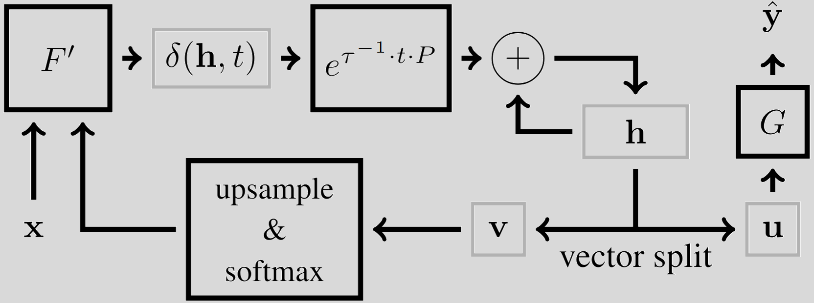
Each iteration updates the internal state using a deep neural network and an exponential decay mechanism. This decay mimics a kind of damping, ensuring the system doesn’t spiral out of control but instead stabilizes over time.

Internal state is updated using a deep neural network, \( F' \), and an exponential decay mechanism. This decay mimics a kind of damping, ensuring the system doesn’t spiral out of control and instead stabilizes over time.

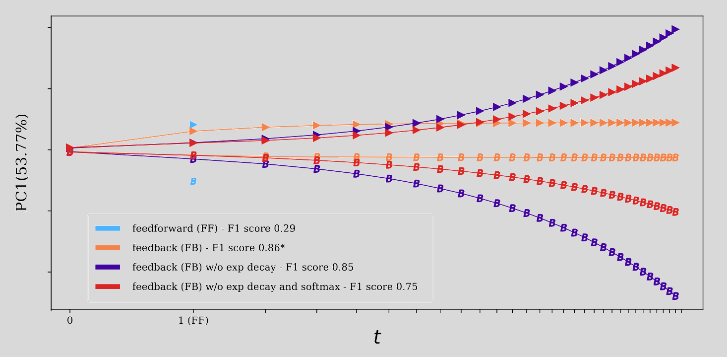
To make this methodology work at scale, i.e. able to learn on ImageNet, we added a few stability tools, namely:

• Softmax projection: ensures that feedback values are bounded and interpretable.
• Exponential decay: gradually dampens updates, allowing the system to settle.
• Orthogonal updates (via QR decomposition): prevent exploding/vanishing gradients when learning the decay dynamics.

This combination makes DFMs biologically inspired and practical to train, even on large datasets.

Converting your neural network to a Deep Feedback Model

In this section, we will go through the code on how to setup a DFM from scratch, using a Resnet. Below is the code for a Resnet. This code was copied from the torchvision implementation of the Resnet, but beware that we omitted code that we thought was unnecessary to understand how to code a DFM.

class _ResNet(nn.Module):
    def __init__(self,**kwargs)
        

        self.frontend=nn.Sequential([nn.Conv2d(3, self.inplanes, kernel_size=7, stride=2, padding=3, bias=False),norm_layer(self.inplanes),nn.ReLU(inplace=True),nn.MaxPool2d(kernel_size=3, stride=2, padding=1)])
        self.layer1 = self._make_layer(block, 64, layers[0])
        self.layer2 = self._make_layer(block, 128, layers[1], stride=2, dilate=replace_stride_with_dilation[0])
        self.layer3 = self._make_layer(block, 256, layers[2], stride=2, dilate=replace_stride_with_dilation[1])
        self.layer4 = self._make_layer(block, 512, layers[3], stride=2, dilate=replace_stride_with_dilation[2])
        self.G=nn.Sequential([nn.AdaptiveAvgPool2d((1, 1)),nn.Linear(512 * block.expansion, num_classes)])

    def forward(self, x):
        x = self.frontend(x)

        x = self.layer1(x)
        x = self.layer2(x)
        x = self.layer3(x)
        x = self.layer4(x)

        return self.G(x)

A Resnet is characterized by 4 layer blocks, a frontend (that has a convolutional layer and max pool), and a classification head (which is our \(G\)).

Now using our python package, dfbmodels, let's go through the code of the corresponding resnet turned into a DFM. Please note that there is a lot of code that is important and is not being shown in this blog post. If you want more details, please visit our github repo.

from dfbmodels.state import StateExpDecay

from dfbmodels.equilibrium import EquilibriumModel

class ResNetDFM(_ResNet, EquilibriumModel):
  def __init__(self, **kwargs):

    self.inplanes=64+(feedback_filters)*self.block_expansion
    self.layer1=self._make_layer(block,64, layers[0])
    self.layer2=self._make_layer(block,128, layers[1], stride=2)
    self.layer3=self._make_layer(block,256, layers[2], stride=2)
    self.layer4=self._make_layer(block,512+feedback_filters, layers[3], stride=2)

    self.G=torch.nn.Sequential(*[self.avgpool, torch.nn.Flatten(start_dim=1), torch.nn.Linear(512 * self.block_expansion, n_classes)])

    self.error_head=StateExpDecay(class_filters+feedback_filters, (shape[0]//4, shape[1]//4))
  
  def step(self, x):
    t=self.T
    
    x=self.layer1(torch.concat((x, self.inlayer1), dim=1))
    x=self.layer2(x)
    x=self.layer3(x)
    x=self.layer4(x)
    
    self.state=self.state+self.error_head(x, T=self.T)

    torch.nn.init.constant_(self.T, self.T+1)
  
  def forward(self, x, T=5):
    x=self.frontend(x)
    
    self.to_equilibrium(x, None, None, T=T-1, atol=atol)

    self.step(x)
    
    return self.prediction()

So we define the layer blocks, just as done in the init function of the original Resnet code, but this time we need to accommodate the number of feedback neurons that are used. We also need to add a layer that performs exponential decay, which is referred to as StateExpDecay.

In the forward pass, the input is processed by the frontend and then it is iteratively looped in the layer blocks. This is done inside the to_equilibrium method that calls step method multiple times. Then at the end the prediction method calls the classification head \(G\).

In order to turn your custom model to a DFM, you just need to identify the frontend (if it has any), and the classification head!

How It Works: Feedback in Action

From what we have seen so far, we are defining DFMs as models that take multiple steps, starting from a blank slate (can be either zeros or random), and it iteratively updates it using feedback from its own predictions. These can be used in classification tasks and segmentation. We argue that there are more applications, but only these two were considered in our experiments. So we have two tasks:

• Semantic segmentation: artificial data of triangle shapes and COCOStuff;
• Object recognition: ImageNet;

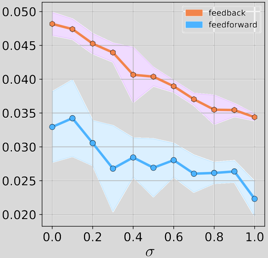
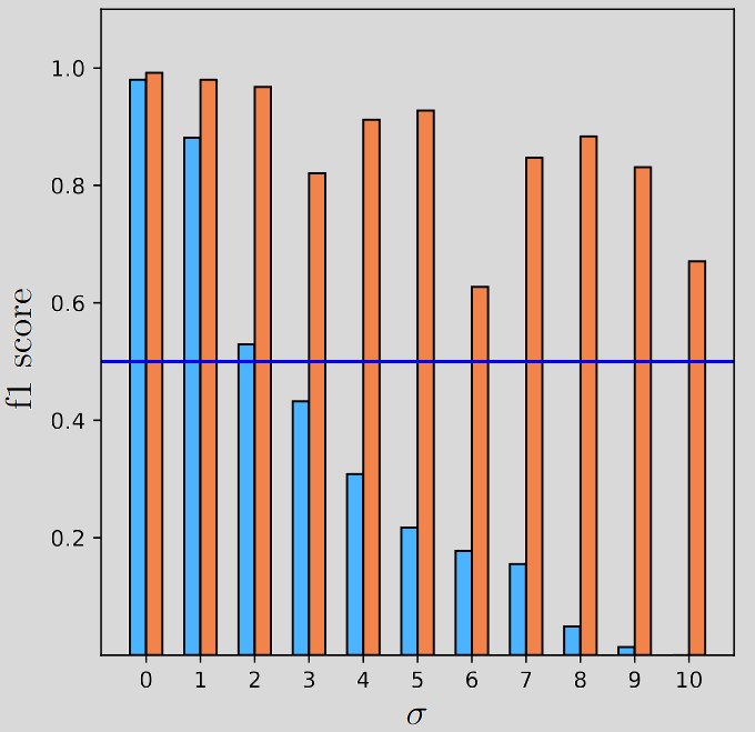
Below are the plots regarding the noise robustness.

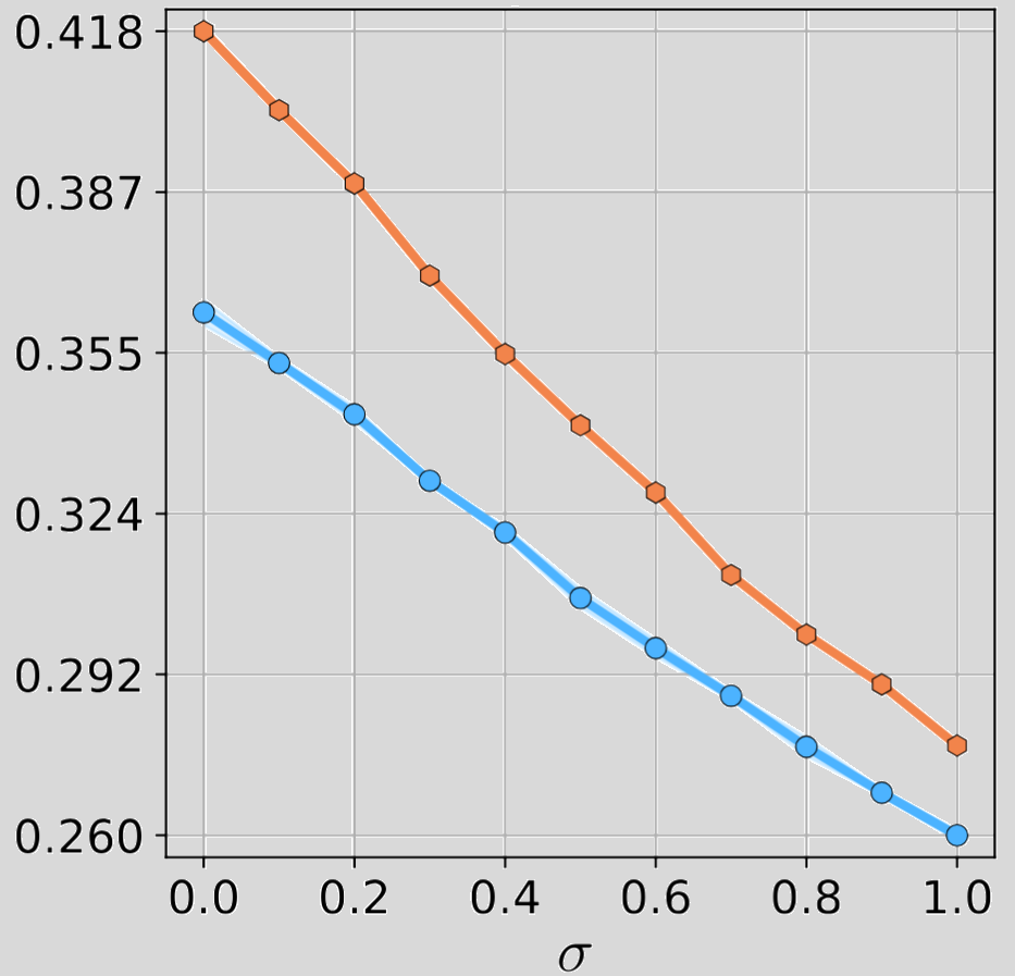
Below are the plots regarding the number of examples analysis that pertains to generalization ability.

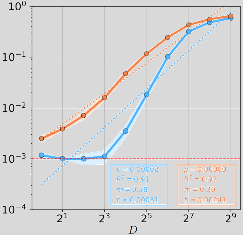
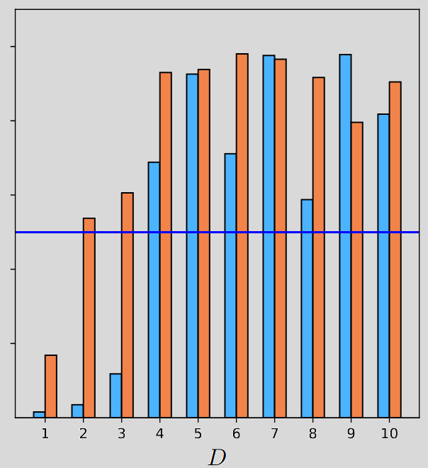
As you can see there is a clear superiority of DFMs against their feedforward counterparts, both in terms of robustness and generalization abilities.

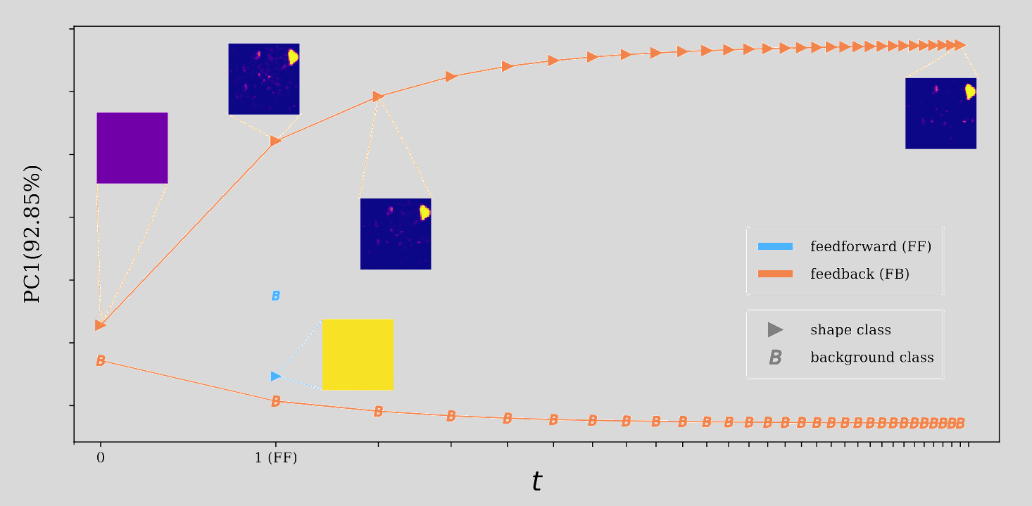
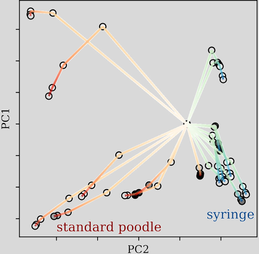
Below we show how DFMs process noisy images. DFMs evolve over time and this gives the model the ability to think.

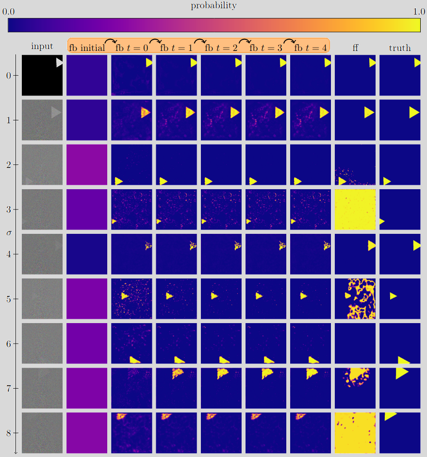
It is very clear in the image above that, with the noise set to \( \sigma=7 \), the model is able to take small steps towards a truthful prediction and kind of correcting the first iteration prediction that is far away from the actual ground truth.

Final remarks

Over the past months at the MLKD lab, we explored a simple but powerful idea that giving deep learning models the ability to revise their own predictions through feedback.

Here's what we found:

• DFMs consistently outperform feedforward baselines, especially in noisy or low data settings;
• Tools like softmax projection, exponential decay, and orthogonality not only ensure convergence, they also make feedback practical to train on large scale data;
• Optimization of the full decision trajectory, not just the final prediction, we tap into dynamics that static models simply do not capture.

Questions?

Please contact me at david DOT calhas AT tecnico DOT ulisboa DOT pt. If you have a question I will happily get back to as soon as I can.

Please visit the youtube video on DFMs. This page does not allow comments, but please feel free to drop a comment on the youtube video page.

Show video